Inference Methods

SAMUEL accumulate the knowledge evidences(for example, scores of activities) to infer the student' knowledge. This accumulation can be configured in different ways which will be explained below.

The operations of SAMUEL web service which get the student model (requestKnowledge and requestKnowledgeWeighted) have, among others, the next parameters:

• date: Student Model date.
• windowSize: Window size (days or evidences number, depending of the parameter windowType) which we assume that student's knowledge doesn't change.
• windowType: Kind of window: 1 to window kind evidences number and 2 to window kind number of days.
• method: Method of evidences accumulation (inference): 1 to Graded Response Model and 2 to Bayes.

For example, if we want to get the today's student model using the evidences of the last 7 days, we'll use date=today's date, windowSize=7 y windowType=2:

On the other hand, if we want to get the today's student model using the last 5 evidences, we'll use date=today's date, windowSize=5 y windowType=1:

Finally, the method parameter shows the accumulation evidences method which will be used by SAMUEL to infer the student model from evidences filtered by the above parameters. In version 1.1 of SAMUEL, the accumulation method available is Graded Response Model(method=1), which will be explained in the next section.

Graded Response Model

Graded Response Model (GRM) is a IRT model for item responses with more than 2 categories (ordered) of responses depending on the degree of resolution of the problem. For each item i there is a number of categories of responses equals to k_i.

• θ is the latent trait.
• X_i is the random variable which indicates the response to graduaded item i.
• x = 0,..,k_i are the current responses.

We want to get:

P_ix(θ) = P_i(X = x | θ)

That is to say, the probability of getting the response x (grade) in the item i (activity) having a knowledge θ. This probability is calculated in two steps:

• Calculation of the "Operating Characteristic Curves" (OCC).

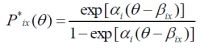
There are k_i curves of the form:

• where P^*_ix = P_i(X ≥ x | θ), for x=1,..,k_i-1 i.e. the probability of getting a grade greater than or equal to x having a knowledge equals to θ.
• α: item discrimination.
• β: k_i -1 difficulty parameters.
• by definition, P^*_i0=1 and P^*_iki=0.
  • Example: for α_j = 1.5, β_j1 = -1.5, β_j2 = -0.5, β_j3 = 0.5, β_j4 = 1.5
    

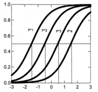
• Calculation of the "Category Response Curves" (CRC).

Once estimated the k_i-1 OCC curves, the probability of responding in the categories (grades) x=0,1,...,k_i-1 is calculated as: P_ix(θ) = P^*_ix(θ)-P^*_ix+1(θ)

• Example:
  

GRM en SAMUEL

The main problem of GRM is to determine the parameters α and β. There are algorithms which use maximum likelihood methods to fit α and β parameters, but to do that it would be needed to have, for each activity, a large enough set of previous students' scores.

In the current version of SAMUEL, the α parameter is a configuration parameter and the parameter β is determinated by a heurísic which depends on the difficulty of the activity, which is set by the teacher. For example, to activities with 5 possibles grades (0...4) SAMUEL would generate the next OCC for α = 1.5 and θ between -3 and 3:

.

Getting the next CRC:

Finally, we have a bayesian network which is configurated with the CRC probabilities. So, SAMUEL infers the student model by calculating the posterior probabilities from the differents activities evidences and assuming an equiprobable initial model: